Mastering data validation in Excel is tricky. However, when you incorporate advanced techniques and formulas, all the data-related work becomes smoother. With exceltopdftricks.com, we ensure your data analysis tricks no longer give you jitters.
Whether you are new or experienced, with knowledge of Excel formulas/tricks, your ability to analyze data will be drastically improved. Mastering the use of Excel enhances not only your skills in data analysis but also renders – an indispensable asset to any organization.
Come along with and read this blog to explore what Excel Formula/Tricks is, how to build it in best-practice ways, important keyboard shortcuts, and some advanced tips to develop mastery of the Excel game.
What are Excel formulas?
Simply put, Excel formulas are equations that perform mathematical calculations on your data. They usually begin with an equal (=) sign and include a mix of values, references to cells, operators, and even functions. For example, the formula (= A1+B1) adds the value of the cell A1 plus B1. It supports all kinds of functions-from simple arithmetic to complex statistical analysis.
Excel Formulas for Beginners
Learners should start from scratch to slowly master the skill of navigation. Here we have provided some basic Excel formula tricks for beginners to get started with.
- Addition: =A1 + B1
- Subtraction: =A1 – B1
- Multiplication: =A1 * B1
- Division: =A1 / B1
- Average: =AVERAGE(A1:A10)
- Sum: =SUM(A1:A10)
- Count: =COUNT(A1:A10)
- Maximum: =MAX(A1:A10)
- Minimum: =MIN(A1:A10)
Our Experts Bring You The Best Practices for Creating formulas
- Use cell reference – Use cell reference to make the formulas dynamic. This will automatically update your formula if the data in the referenced cell changes.
- Keep it simple – Break down complex calculations into smaller and simpler parts to understand and incorporate them.
- Use named ranges – Assign names to the range of cells to make your formulas more readable. For example, if you name a range of sales data “SalesData”, you can use =SUM(SalesData).
- Document your formulas – Add comments or notes to the spreadsheet for complex formulas, especially useful for a collaborative environment.
- Test your formulas – Test the formulas with known values to ensure accuracy.
Excel keyboard Shortcuts
Keyboard shortcuts speed up your workflow, hence, keyboard shortcuts are essential for mastering Excel formula/tricks. Here are some keyboard shortcuts for you.
- Ctrl + C: Copy
- Ctrl + V: Paste
- Ctrl + Z: Undo
- Ctrl + Y: Redo
- Ctrl + A: Select all
- Ctrl + F: Find
- Ctrl + H: Replace
- Alt + E, S, V: Paste Special
- F2: Edit the active cell
- Shift + Space: Select the entire row
- Ctrl + Space: Select the entire column
- Alt + Enter: Start a new line within a cell
Top 30 Advanced Excel Formula/Tricks
Everyone should master Excel formulas to make their task easier and smoother. Here are the Top 30 advanced Excel tips and tricks.
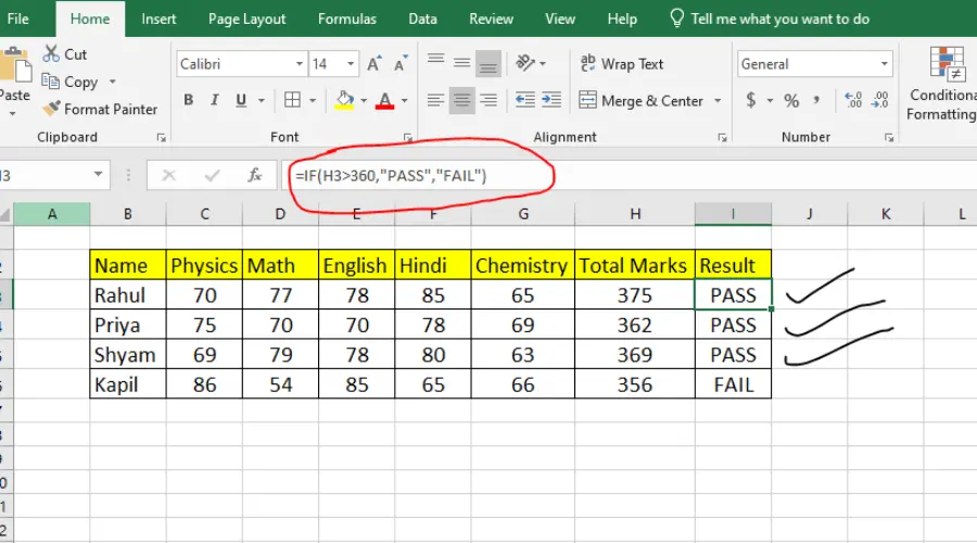
- Use IF Statements: Data flow can be controlled with conditional formulas. Example: =IF(A1 > 10, “Yes”, “No”).
- VLOOKUP: VLOOKUP helps search for an item in the table and get a value for that item from a specific column. Example: =VLOOKUP(A1, B1:D10, 2, FALSE).
- INDEX and MATCH: An advanced form of VLOOKUP that accomplishes the same task but with more versatility. =INDEX(B1:B10, MATCH(A1, A1:A10, 0)).
- Conditional Formatting: Enables color cells depending on specific conditions, displaying a trend in the data. Go to Home > Conditional Formatting.
- Pivot Tables: Difficult sets of data can be summarized using Pivot Tables (Insert > Pivot Table).
- Data Validation: Prevents the entry of incorrect data into the cell through validation rules (Data > Data Validation).
- Dynamic Arrays: Functions like FILTER, SORT, AND UNIQUE are employed to successfully deal with arrays.
- Power Query: Power Query efficiently transforms data. (Data > Get & Transform).
- Text Functions: The most common operations are presented, such as manipulations with strings like LEFT, RIGHT, MID, TRIM, and CONCATENATE.
- Date Functions: Use functions like TODAY(), NOW(), DATEDIF, and EDATE for date calculations.
- Goal Seek: When provided with a desired result, calculate the input value for that result to occur (Data > What-If Analysis > Goal Seek).
- SUMIF and SUMIFS: Conditional summation of various ranges using conditions. Example: =SUMIF(A1:A10, “>10”, B1:B10).
- COUNTIF and COUNTIFS: Counters based on conditions imposed. Example: =COUNTIF(A1:A10, “Yes”).
- Remove Duplicates: Clean your Data by Removing Duplicates (Data > Remove Duplicates).
- Flash Fill: Automatically fills data based on patterns (Data > Flash Fill).
- Freeze Panes: Certain rows or columns are marked to remain in view when the user scrolls down or sideways (View > Freeze Panes).
- Transpose Data: The Paste Special command copies data across the columns rather than filling a row with column data.
- What-If Analysis: Alternative outcomes, or scenarios, with the aid of the Scenario Manager tool, are investigated under the Data sub-section and What-If analysis section. (Data > What-If Analysis).
- Sparkline Charts: Miniature charts embedded in a single cell to demonstrate data variations (Insert > Sparklines).
- Hyperlinks: Add hyperlinks to other websites or documents wherever required.
- Comments and Notes: Introduce comments during the editing process or leave a comment for prospective users.
- Custom Number Formats: Modify how the platform displays digits without altering their actual values.
- Chart Creation: Charts are used to make data easier to understand (Insert > Chart).
- Group and Outline: This feature combines and simplifies data into markable areas upon which users can click to reveal or hide information (Data > Group).
- Keyboard Shortcuts for Formulas: The F4 key cycles among relative cell references in a formula. (absolute/relative).
- Use Arrays: Get used to array formulas for complex computations.
- Data Tables: Construct a data table to observe the changing result, either on one or two parameters (Data > What-If Analysis > Data Table).
- Named Formula: Name the formulas to enhance the utilization.
- Conditional IFERROR: Minimizes error risks in the process of carrying out calculations. Example: =IFERROR(A1/B1, “Error”).
- Using the Watch Window: Keep track of certain cells without changing the currently active section of the workbook (Formulas > Watch Window).