Index Match combination in Excel is useful for various kinds of lookups to get the preferable data in Excel spreadsheets. These functions allow you to easily find the data in your datasheet through different lookups, including horizontal and vertical lookups, 2-way lookups, left lookups, case-sensitive lookups, etc. For professionals whose daily work involves the use of Excel for various purposes, learning index match formulas in Excel can be highly beneficial. Besides, It makes the process of navigating through complex data seamless.
If you want to know the hidden secrets of Index Match in Excel and how you can make use of them to boost your work efficiency, get into this blog as here, we are covering a detailed guide to using Index Match in Excel. First, we will cover the INDEX and MATCH separately and then will present the usage of a combination of two functions to form a two-way lookup.
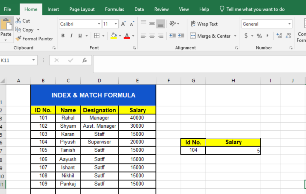
Understanding the INDEX Function in Excel
The INDEX function is a dynamic tool in Excel that recovers the value in a specified location. It features the content in a cell, defined by relative row and column. It allows you to quickly get the information on your spreadsheet. Irrespective of how massive the list or table is, you can easily find the data you are looking for. From getting a name in a long list to a particular figure in a budget, it helps you figure out the desired information instantly.
The first step in using INDEX is to provide the array or range, which you expect involves your answer. After that, you are required to define the row and column to get the correct value. Within the INDEX range, you can move anywhere.
INDEX formula in Excel
The Syntax of INDEX function in Excel is =INDEX(array, row_num, [column_num])

The dimensions of the INDEX function in Excel:
- array: Array is the range that contains the retrieved value. Here, you direct towards the block of cells to signify that the desired information belongs to this area.
- row_num: Through row_num, you can specify the rows to the INDEX function to go from the selected area to locate the specific row to feature the data. If you specify “3”, INDEX will go two rows down from the top of the selected area and show you the related data.
- [column_num]: Just like above, here you will be specifying the column to the INDEX function to move to the right side towards the entered column. If you specify “5”, it will show the data by directing to the 5th position rightwards in the columns.
To sum up, the function of Excel INDEX works like this “In the specified block of cells, move down the defined row and move right towards the specified columns, and unveil the value.” This is how you use the INDEX formula to get the desired data.
Steps to use the INDEX Function in Excel:
To use the INDEX function in Excel effortlessly, check out the steps given in the guide “How to use INDEX in Excel” below:
- Choose the range/ array: In the first step, select the area you are certain, including your desired data.
- Choose the Row Number: Then, fill in the row number that comprises your data.
- Choose the Column Number: If your range houses more columns, you can mention the column number to specify the particular cell.
Downsides
No doubt, INDEX in Excel is a flexible tool useful to navigate the data. However, it has some limitations as It’s difficult to remember the exact row and column numbers in a large spreadsheet, involving numerous rows and columns. Thus, getting the data in such data sheets is a complex task.
Exploring Match Function in Excel
The functions of Match in Excel are a bit like the function of Index with a varied formula. This tool takes you to reach the position of the desired value of the row, column, or range. In VLOOKUP or HLOOKUP, you get the retrieved original data, however, in Match Excel, you get the relative position of the cell. One of its exclusive properties is its case insensitive, functioning aptly in horizontal and vertical ranges.
So, now, getting information in any big list, including names or numbers is not an uphill battle as you can find a particular item quickly with the MATCH tool. As per your entered details in the formula or function, it will leaf through the data and provide you the precise information. Thus it not only saves your time in running your eye over the comprehensive data but also ensures the accuracy of the cell in the list or table.
Match Function Formula
To create a match function, you are required to enter =MATCH(lookup_value, lookup_array, [match_type]).

Parts of the Excel INDEX function:
Here, we have broken down the parts of the INDEX function to make you familiar with each segment effectively.
- lookup_value: It refers to the information in terms of the value you are searching for. For this, you can direct towards the cell that accommodates this value or enter it directly into the stated formula.
- lookup_array: This segment points to the list or table in your datasheet which contains your value or item as you expect.
- match_type: In this place, using “0” tells that you are seeking the exact match, which indicates the MATCH function that your desired information should accurately match the lookup value.
How to Use the MATCH Function in Excel?
Using the MATCH Function in Excel is seamless with simple steps to go through. Look at the steps mentioned below to utilize this tool with no trouble.
- Selection of the Lookup Value: Pick out the value you want to find out. It can be a number, text, or a cell reference.
- Choosing Lookup Range: Then, in the second step, select the range (row or column) to specify the MATCH function to scan the lookup value in the sheet.
- Choose the Match Type:
- If you want to get an exact match, enter 0.
- To get a related match in ascending arrangement, enter 1.
- To get a related match in descending order, enter -1.
Using the MATCH Function for Multiple Metrics
If you want to use the function of MATCH for numerous criteria, your formula should be one-headed. To do this, you need to combine MATCH with another INDEX function. You can also choose to change your formula. In this way, Excel will consider it as a distinct range formula.
Utilizing the combination of INDEX MATCH Function
Using INDEX and MATCH together in Excel is an effective way for data lookups. Through the Index function, you can utilize static row and column numbers and through the MATCH function, you can locate the positions of rows and columns depending upon the particular criteria. Thus, the INDEX MATCH Combination addresses the shortcomings of VLOOKUP perfectly.
Besides, the INDEX MATCH combination allows you to do a “left lookup”. Thus, you can extract the row position of a value using any property at the right. For instance, there is a list of a few items, including costs on the right side. So suppose you bought a thing worth cost Rs. 100. As the price of the item, 100 Rs. is known, the item can be extracted easily from the right side. In the case of VLOOKUP, you can’t get the left side of the costs of items.
Formula to use INDEX MATCH Excel Functions Together:
=INDEX(array, MATCH(lookup_value, lookup_array, [match_type]), MATCH(lookup_value, lookup_array, [match_type]))

Characteristics of INDEX MATCH in Excel
There are various characteristics of INDEX MATCH in Excel that make them powerful tools to use.
- Left Lookup: Through the INDEX MATCH combination, left lookup can be applied, unlike VLOOKUP.
- Case-Sensitive: The MATCH function in Excel is not case-sensitive so if you want to perform a case-sensitive lookup, you need to use the EXACT function with MATCH. The MATCH function doesn’t work case-sensitive by default. For example: If there is the term “ANALYSIS” in the data sheet and you used the MATCH function with either Analysis, analysis, analysis, it will show the row position of ANALYSIS. By using the EXACT function with INDEX and MATCH, you can make it case-sensitive.
- INDEX MATCH Multiple Criteria Lookup: Multiple criteria lookup means a lookup that shows similarity to more than one column simultaneously.
- Usage in varied sheets: For recovering the data from the distinct sheet through the INDEX MATCH combination, you are required to reference the sheet name in the framework. Following this, you need to look for the data in one sheet and get it in another, thus it functions as a useful tool for analyzing the multi-sheet data.
The syntax for using INDEX and MATCH Across different Sheets:
- =INDEX(SheetName!Range, MATCH(LookupValue, SheetName!LookupRange, MatchType))
- Sheet 1 is the sheet where you want to see the result.
- Sheet 2 records the data.
What are the benefits of INDEX MATCH Functions?
INDEX and MATCH functions in Excel sheets are beneficial for various reasons that are listed below:
- Flexible functions: These functions enable you to perform a lookup in any direction either left, right, up, or down.
- Case-Sensitive: You can perform the Case-sensitive lookups conveniently by combining the EXACT function with the MATCH function.
- Adaptive: INDEX and MATCH functions are adaptive, that fit according to the changes in the data structure.
- Multiple criteria: By using the INDEX and MATCH functions combination, you can navigate to the complex lookups easily.
Key Takeaways
Gaining proficiency in INDEX and MATCH functions will help you handle the complex data in the broad Excel spreadsheets with no hurdle. Through these flexible and dynamic functions, you can delve into the advanced lookups, letting you find the data from anywhere in the sheets. Thus, these functions serve as key tools for professionals dealing with large datasheets, enhancing their productivity and work efficiency.
Related Links
| ROUND Function In Excel | How to Convert PDF to Excel |
| Top 30 Excel Formulas/Tricks Guide | XLOOKUP Function in Excel |
FAQs
Q.1. How to apply an INDEX MATCH in Excel?
A.1. To apply an INDEX MATCH in Excel, you need to look for the lookup value by column and row numbers through the INDEX function column and then you will get those numbers through the MATCH function.The formula to use INDEX MATCH in excel is INDEX(array, MATCH(lookup_value, lookup_array, [match_type]), MATCH(lookup_value, lookup_array, [match_type])).
Q.2. Is the INDEX MATCH better than VLOOKUP?
A.2. INDEX/MATCH is better than VLOOKUP as you can move columns easily without spoiling your results, unlike VLOOKUP which showcases inaccurate results in the case of moving columns.
Q.3. How to use the match function in Excel?
A.3. To use the MATCH function in Excel, apply the formula =MATCH(lookup_value, lookup_array, [match_type]). After the application of the formula, the INDEX function will find the particular data in a range of cells and retrieve the relative position of that item in the range.
Q.4. Which is faster, VLOOKUP or INDEX match?
A.4. Considering the factors of finding accurate data, INDEX-MATCH is 13% more expeditious than VLOOKUP.